

What is the necessity of fine tuning?
Pre-trained large language models undergo extensive training on vast data from the internet, resulting in exceptional performance across a broad spectrum of tasks. Nonetheless, in most real-world scenarios, there arises a necessity for the model to possess expertise in a particular, specialized domain. Numerous applications in the fields of natural language processing and computer vision rely on the adaptation of a single large-scale, pre-trained language model for multiple downstream applications. This adaptation process is typically achieved through a technique called fine-tuning, which involves customizing the model to a specific domain and task. Consequently, fine-tuning the model becomes vital to achieve highest levels of performance and efficiency on downstream tasks. The pre-trained models serve as a robust foundation for the fine-tuning process which is specifically tailored to address targeted tasks.
What is the conventional way of fine-tuning?
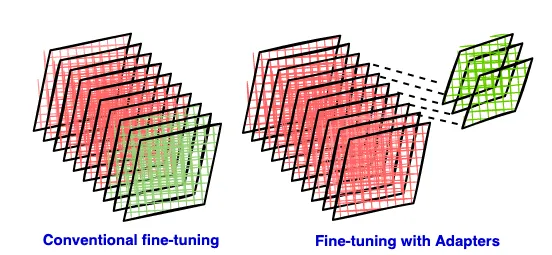
During the conventional fine-tuning of deep neural networks, modifications are applied to the top layers of the network, while the lower layers remain fixed or “frozen”. This is necessary because the label spaces and loss functions for downstream tasks often differ from those of the original pre-trained model. However, a notable drawback of this approach is that the resulting new model retains the same number of parameters as the original model, which can be quite substantial. Nonetheless, creating a separate full model for each downstream task may not be efficient when working with contemporary large language models (LLMs).
In many cases, both the top layers and the original weights undergo co-training. LLMs have grown to such immense sizes that computational demands of fine-tuning all the parameters of the model is resource intensive and prohibitively costly. Additionally, concerns arise about the availability of an adequate amount of labeled data for effective training without over-fitting.
How can fine-tuning be made efficient?
Many sought to mitigate this by learning a set of few extra parameters for each new task. This way, we only need to store and load a small number of task-specific parameters in addition to the pre-trained model for each task, greatly boosting the operational efficiency when deployed. This is one of the Parameter-Efficient Fine-Tuning (PEFT) methods and it focuses on fine-tuning only the external modules called Adapters. This approach significantly reduces computational and storage costs.
The advantages of employing parameter-efficient methods for fine-tuning can be articulated in two aspects:
- Regarding disk storage: Fine-tuning solely an adapter module with a limited number of additional parameters necessitates storing only the adapter for each downstream task. This significantly reduces the required storage space for models. It prompts the question of whether maintaining an entire additional copy of LLaMA for each distinct sub-task is truly necessary.
- Concerning RAM: While the exact measurement of the memory footprint considers factors like batch size and various buffers needed during training, the general memory requirement is roughly four times the size of the model. This accounts for gradients, activations, and other elements for each parameter. Fine-tuning a smaller set of parameters alleviates the need to maintain optimizer states for the majority of parameters. During the forward pass, frozen layer weights are used to compute the loss without storing local gradients, saving memory by eliminating the need to save gradients for these layers. During the backward pass, the weights of the frozen layers remain unchanged, which also saves computational resources and RAM, as no calculations are needed for updating these weights.
What are adapters and how are they used for fine-tuning?
Adapter modules, as detailed in the paper by Houlsby et al.¹, involve making minor architectural adjustments to repurpose a pre-trained network for a downstream task. Specifically, the adapter tuning strategy entails introducing new layers into the original network. In the fine-tuning process, the original network’s weights are kept frozen, allowing only the new adapter layers to be trained, enabling the unchanged network parameters of original network to be shared across multiple tasks. LoRA (Low-Rank Adaptation), is a type of adapter technique which refers to a method of inserting low-rank matrices as adapters.
Adapter modules possess two key characteristics:
- Adapter modules are relatively smaller than the layers of the original network.
- Their initialization ensures minimal disruption to training performance in the early stages, allowing the training behavior to closely resemble that of the original model while gradually adapting to the downstream task.
How can fewer parameters be enough for fine-tuning?
Normally, training a model with hundreds of millions of parameters requires a lot of data. Otherwise, the model might ‘over-fit’ — it would perform well on its training data but poorly on new, unseen data. However, these large language models can be fine-tuned with surprisingly small datasets while still maintaining good performance. This raises a question: how is this possible?
Li et al.² and Aghajanyan et al.³ showed that the learned over-parametrized models in fact reside on a low intrinsic dimension. This line prompts further questions regarding learned over parameterized models, model dimensions, visualizing objective function in a certain space, dimension of an objective function, intrinsic dimension (ID) of an objective function, its significance, If ID was so low why do we have such large networks in the first place?, and the method used to calculate it, which I will attempt to address in another article.
To pave the way for our discussion on LoRA, here is a quick summary — While deep networks may have a large number of parameters, say ’n’, only a small subset of these, say ‘d’ where d<<n, truly influences the learning process Li et al.² The remaining parameters introduce additional dimensions to the solution space, simplifying the training process. The abundant solution space facilitates smoother convergence. ‘d’ represents what they call the model’s intrinsic dimension for that particular task.
Aghajanyan et al.³ tried to explore fine tuning in the lens of intrinsic dimension and observed that (1) Pre-training effectively compresses the knowledge and the ability of compressing knowledge gets better with longer pre-training time and (2) Larger models can learn better representation of the training data.
This means that larger models, after pre-training, are easier to fine-tune effectively with less data. When fine-tuning on the MRCP⁵ dataset, authors found that using RoBERTa⁴ Large’s full capacity of 354 million parameters (n) resulted in a performance similar to a scenario where they fine-tuned the same model using only 207 (d) parameters.
Adapter modules are dense layers introduced between the existing layers of the pre-trained base model which we can refer to as ‘adoptee layers,’ as in this article⁶. In Part-2, we will explore how adapters integrate into the overall architecture that includes the base model. Taking inspiration from the above works, authors of LoRA⁸ hypothesized that the adapter modules (new weight matrix for the adapted task) can be decomposed into low-rank matrices which have a very low “intrinsic rank”. They proposed that pre-trained large language models have a low “intrinsic dimension” when they are adapted to a new task. Taking GPT-3, 175 billion parameters as an illustration, the authors demonstrated that an extremely low rank (referred to as ‘r,’ which can be as low as one or two) is sufficient, even when the full rank (‘d’) reaches as high as 12,288, making LoRA both storage and compute efficient.
The Idea Behind Low-Rank Adaptation
Consider a matrix, denoted as A, with dimensions p x q, which holds certain information. The rank of a matrix is defined as the highest number of linearly independent rows or columns it contains. A concept often introduced in school is that the rank can be easily determined from the matrix’s echelon form. When the rank of matrix A, denoted as r, is less than both p and q, such matrices are termed “rank deficient.” This implies that a full-sized matrix (p x q) isn’t necessary to convey all the information, as it includes a significant amount of redundancy. Consequently, the same information could be conveyed using fewer parameters. In the field of machine learning, its common to work with matrices that are approximated with lower ranks, carrying information in a more condensed form.
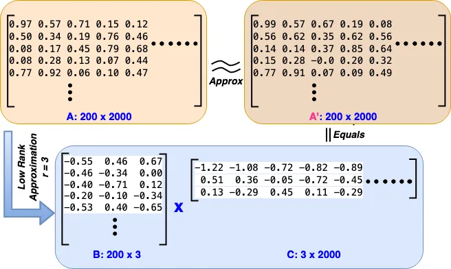
Methods for low-rank approximation aim to approximate a matrix A with a another matrix of lower rank. The objective is to identify matrices B and C, where the product of B and C approximates A (A_pxq ≈ B_pxr × C_rxq), and both B and C have ranks lower than A. We can even pre-define a rank r and accordingly determine B and C. Typically p x r + r x q << p x q , indicating that significantly less space is needed to store the same information. This principle is widely utilized in data compression applications. It’s possible to choose an r that is smaller than the actual rank of A, yet construct B and C in a way that their product approximately resembles A, effectively capturing the essential information. This approach represents a balance between retaining important information and managing spatial constraints in data representation. The reduced number of rows and columns that encapsulate the essential information in a dataset are often referred to as the key features of the data. Singular Value Decomposition (SVD) is the technique employed to identify such matrices B and C for a given matrix A.
The authors of LoRA hypothesize that adapters (weight update matrices) have a low intrinsic rank which refers to the idea that the information contained within the matrix can be represented using fewer dimensions than the the adaptee matrix/layer of the base model might suggest.
Rather than decomposing the selected adaptee matrices through SVD, LoRA focuses on learning the low-rank adapter matrices B and C, for a given specific downstream task.
In our case A_pxq = W_2000x200, B = lora_A and C = lora_B. We approximate a high-dimensional matrix or dataset using a lower-dimensional representation. In other words, we try to find a (linear) combination of a small number of dimensions in the original feature space (or matrix) that can capture most of the information in the dataset. Opting for a smaller r leads to more compact low rank matrices (Adapters), which in turn require less storage space and involve fewer computations, thereby accelerating the fine-tuning process. However, the capacity for adaptation to new tasks might be compromised. Thus, there’s a trade-off between reducing space-time complexity and maintaining the ability to adapt effectively to subsequent tasks.
In Part-2 of the blog series, we will analyze LoRA through its implementation on a Multilayer Perceptron (MLP). It commences with setting the stage for fine-tuning by creating a toy dataset for a binary classification task. Following this, the blog delves into the core of fine-tuning with LoRA, detailing the process of adapter insertion, parameter configuration, and assessing the resulting parameter efficiency, which underscores LoRA’s capability to mitigate computational and storage demands. Practical considerations for sharing and loading models through the Hugging Face Hub are discussed, enhancing the utility and accessibility of fine-tuned models. Finally, the blog addresses LoRA’s limitations in memory usage during inference and proposes solutions like QLoRA, rounding off the discussion with a comprehensive look at managing and optimizing LLMs for specific tasks with minimal resource overhead.
Thanks to my colleagues at Sahaj for all the brainstorming sessions.
All images are by the author unless otherwise stated.
[7] Parameter-Efficient LLM Finetuning With Low-Rank Adaptation (LoRA)

