
“Instead of tweaking all weights, we project into a compact subspace and optimize just a few directions that matter.”
In Part I of this series, we delved into the concept of Intrinsic Dimension (ID) and its implications on fine-tuning. To recap, the intrinsic dimension of an objective function measures the minimal number of parameters needed to achieve satisfactory performance on a given task (Li et al.,¹). For example, in their seminal work, the authors demonstrated that a fully connected neural network with a total of 199,210 parameters (architecture: 784–200–200–10) achieved a 90% performance threshold (d₉₀) on the MNIST dataset with an intrinsic dimension of only 750 parameters.
A natural follow up question is:
How can we reduce the optimization problem from the full 199,210-parameter space to just 750 dimensions without manually selecting which parameters to keep?
The answer lies in projecting the parameters into a lower-dimensional subspace. Instead of optimizing directly in the high-dimensional parameter space (n-dimensional), the method leverages a random subspace of dimension d to guide the optimization. Most of the original parameters are effectively “frozen,” and only the projected parameters in the reduced subspace are fine-tuned.
Measuring Intrinsic Dimension via Random Subspace Training
In this article, we aim to demystify the process of measuring ID using random subspace training, as described in Section 2 of the referenced paper. The approach prompts a series of questions:
How do we project the base model parameters (of dimension n) into a lower-dimensional space d?
How is this projection integrated into the network’s computation graph to enable proper gradient flow?
Why does this projection-based approach work?
What are alternate methods to work with a lower-dimensional sub-space?
In the following sections, we will systematically explore these questions and replicate the results presented in the original paper (Li et al.,¹).
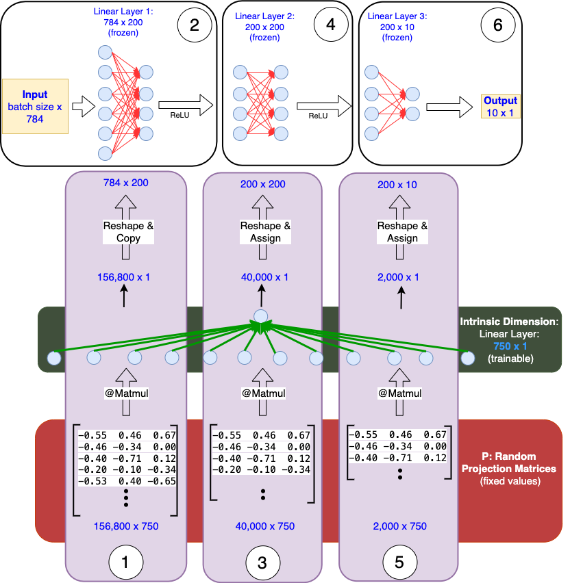
Define the Base model and the Objective function
We begin by implementing a simple Multi-Layer Perceptron (MLP) with the architecture 784–200–200–10 (as mentioned above). The network uses ReLU activation, takes input of dimension 784 (flattened MNIST images), and outputs predictions for 10 classes.
What is the Projection Mechanism?
The core of this method lies in projecting the parameters of the base model into a lower-dimensional subspace: θ(D) = θ₀(D) + P x θ(d)
θ₀(D): Parameters of the base model in the original D-dimensional space (these remain frozen during training).
# Freeze base model parameters
for param in base_model.parameters():
param.requires_grad = Falseθ(d): Parameters in the reduced d-dimensional subspace (the only parameters trained) are initialized to a vector of all zeros, so that initially θ(D) = θ₀(D). These parameters are registered as nn.Parameter, ensuring they are part of the computation graph. Training modifies only these ‘d’ parameters.
# Initialize and register intrinsic parameters
intrinsic_params = nn.Parameter(torch.randn(intrinsic_dim, device=device) * 0.01)
P: Projection matrix maps the base model parameters to the lower-dimensional subspace (Intrinsic Dimension: d). It is fixed and registered as a buffer (not a parameter).
# Create projection matrix
proj_matrix = torch.randn(param_size, intrinsic_dim).to(device) * np.sqrt(1/intrinsic_dim)
Say d = 750, each layer of the base model is projected to a single d-dimensional vector.
— Layer 1 Weights [784, 200] → Flatten: [156800] →P₁: [156800, 750]
— Layer 2 Weights [200, 200] → Flatten: [4000] → P₂: [4000, 750]
— Layer 3 Weights [200, 10] → Flatten: [2000] → P₃: [2000, 750]
Projection Operations for each layer weight:
projected_weight = projection_matrix @ intrinsic_params
Layer 1: [156800, 750] @ [750, 1] → [156800, 1] → [784, 200]
Forward Pass
How are P and θ(d) integrated into the network’s computation graph to enable proper gradient flow?
During the forward pass, the intrinsic parameters are mapped to the base model’s parameter space using the projection matrix via matrix multiplication. This operation ensures proper gradient flow during backpropagation.
# matmul operation connects the intrinsic params to the base model params through proj_matrix
projected_params = torch.matmul(proj_matrix, intrinsic_params)
Layer Operations (using projected weights):
Input: [batch_size, 784]
Layer 1:
- Projection: [156800, 750] @ [750] → [156800] → reshape to [200, 784]
- Forward: [batch_size, 784] @ [200, 784]ᵀ → [batch_size, 200]
- ReLU
Layer 2:
- Projection: [40000, 750] @ [750] → [40000] → reshape to [200, 200]
- Forward: [batch_size, 200] @ [200, 200]ᵀ → [batch_size, 200]
- ReLU
Layer 3:
- Projection: [2000, 750] @ [750] → [2000] → reshape to [10, 200]
- Forward: [batch_size, 200] @ [10, 200]ᵀ → [batch_size, 10]During back propagation, the gradient flow follows this pathway:
loss → layer outputs → projected weights (copied onto the frozen base model parameters) → projection operation (matrix multiplication) → θ(d) (intrinsic parameters).
In the order of operation: 1. Layer_1 projection, 2. Layer_1 forward, 3. Layer_2 projection, 4. Layer_2 forward, 5. Layer_3 projection, 6. Layer_3 forward. Intrinsic Dimension vector of size [750 x 1] is trainable. P is fixed.
To achieve flexibility in dynamically computing the projected weights, use
torch.nn.functional.linear()instead oftorch.nn.Linear().
Why does this Projection-Based approach work?
Random projections enable high-dimensional data to be projected onto a lower-dimensional space while approximately preserving key geometric properties such as:
Euclidean distances between points
Angles between vectors
Inner products
This preservation is crucial for maintaining the model’s learning capacity even in the reduced parameter space.
The Role of the Projection Matrix (P): This matrix defines how movements in the d-dimensional space translate to movements in the D-dimensional space. It serves as a bridge between the reduced and full parameter spaces.
Key characteristics of P:
Unit Vector Columns: Columns of P are normalized to unit length, so steps of unit length in θ(d) chart out unit length motions of θ(D).
Orthogonal Columns: High dimension random vectors are approximately orthogonal, even without explicit orthogonalization.
# Normalize each column to have unit length
proj_matrix = proj_matrix / torch.norm(proj_matrix, dim=0, keepdim=True)
By this construction, P forms an approximately orthonormal basis for a randomly oriented d dimensional subspace of R(D). An orthonormal matrix preserves the above characteristics (distances, angles, and inner products). This approximation suffices for high-dimensional random projections, offering a practical trade-off between computational cost and accuracy.
Results
The fact that 750 parameters can capture the behavior of 200K parameters suggests the optimization landscape itself has a low-dimensional structure.
To store this network, one need to only store a tuple of three items: (i) the random seed to generate the frozen θ₀(D), (ii) the random seed to generate P and (iii) the 750 floating point numbers in θ(d).
Adapter based PEFT techniques draw inspiration from this practical aspect.
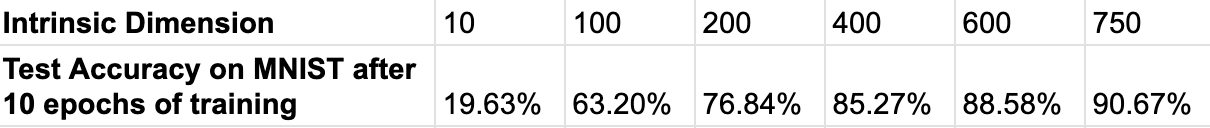
As shown in the table above, we reproduced the results claimed in the Li et al.,¹ paper. By systematically increasing the intrinsic dimension d, we observed that the model achieves 90% accuracy at d = 750, consistent with the findings in the paper.
The code for this experiment is available here, including the implementation to replicate the results by varying d and a mechanism to verify gradient flow within the network.
What are alternate methods to work with a lower-dimension sub-space?
The authors proposed two other variations of the projection matrix P. One notable variation is the Fast-food Transform, which is particularly advantageous for large-scale neural networks because it is memory efficient.
Structure-Aware Intrinsic Dimension (SAID): A projection mechanism which focuses on layers with more task-relevant information (Aghajanyan et al.²).
Pruning: Instead of reducing dimensions through projections, identify the important connections.
[3] Demi Guo, Alexander M. Rush, and Yoon Kim. 2021. Parameter-Efficient Transfer Learning with Diff Pruning.
[4] Max Ploner, Alan Akbik, Parameter-Efficient Fine-Tuning: Is There An Optimal Subset of Parameters to Tune?

