
Understanding the Intrinsic Dimension (ID) of a Model and Why Networks Stay so Large Despite a very Tiny ID
Learned over-parameterized models inherently exist within a low intrinsic dimension {Li et al.¹ and Aghajanyan et al.³}. To understand this concept better, let’s delve into the following questions:
What is a model’s dimension?
What is an Objective function and its landscape?
What is ID and how can it be visualized through graphs of convex and non-convex landscapes?
How do you identify the ID of a network?
If the ID of an objective function is so low, why do we have such large networks in the first place?
How does ID influence fine-tuning?
Why Does This Matter? Where Does It Lead?
What is a model’s dimension?
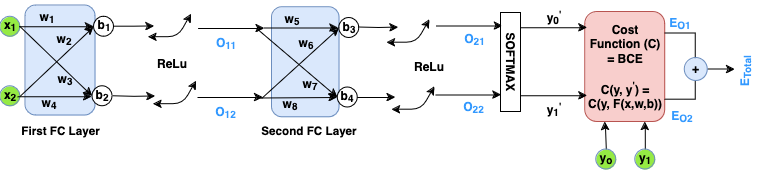
Let’s consider a Multi-Layer Perceptron (MLP) to understand model dimensionality. Our example MLP consists of two Fully Connected (FC) layers with ReLU activations and a final softmax layer for binary classification. In FC layers, which are fundamental to deep learning architectures including transformers, every neuron in the input set connects to every neuron in the output set.
For more details, please refer to the Preliminaries (Chapter 2) of https://github.com/s3pi/Masters-Thesis
The model’s architecture structured as 2–2–2 can be broken down as follows:
First FC Layer:
— 2×2 weight matrix [w₁, w₂, w₃, w₄]
— 2×1 bias matrix [b₁, b₂]
Total parameters: 6Second FC Layer:
— 2×2 weight matrix [w₅, w₆, w₇, w₈]
— 2×1 bias matrix [b₃, b₄]
Total parameters: 6
The model’s dimension is defined by the total number of learnable parameters: 12 (8 weights + 4 biases).
What is an Objective function and its landscape?
Input Data: The input data is represented as [x₁, x₂], with a dimension of 2.
Network architecture: The network can be described as a function parameterized by the input, weights, and biases: F(x, w, b).
Objective function (C): F produces two outputs, y₁’ and y₂’, which are then compared against the ground truth values y₁ and y₂ using the Binary Cross-Entropy (BCE) loss function. The objective function, also known as the Cost Function or Loss function, is represented as C(y, F(x, w, b)). It would calculate the error or loss, measuring how far are the predictions from the actual values. The dimension of the objective function is the same as the dimension of the model, and it corresponds to the total number of learnable parameters within the model.
Objective (Loss) Landscape: The objective function C forms a surface in a 12-dimensional hyperspace, known as the objective landscape. This landscape represents the “shape” of the loss function across different parameter values.
Once the input data, the network architecture and loss are established, the objective landscape (shape of the objective function) is frozen.
Training: Training the network involves navigating this landscape — often visualized as a surface with hills and valleys — to find a point where the loss is minimized. This point, where the loss reaches its lowest value, is known as a local minimum.
While the “hills and valleys” metaphor helps illustrate the concept, the intuition is far from accurate because it’s challenging for us to imagine a hyper space beyond 3 dimensions.
What is Intrinsic Dimension (ID)?
The ID of an objective function measures the minimum number of parameters needed to reach satisfactory solutions to the respective objective (Li et al.,)¹.
If ’n’ represents the total number of parameters in a model, then the objective function forms a specific surface within an ‘n’-dimensional hyperspace. Consider a model with 3 parameters or dimensions (n = 3), which can be visualized in our 3D world and its objective landscape forms a V-shaped valley, with a straight line (ridge or trough) extending infinitely along the y-dimension where the function value is 0, while the rest of the objective function forms a bowl shape.
Let’s denote the parameters of the model as x, y, and z, representing the weights w₁, w₂, w₃, respectively.
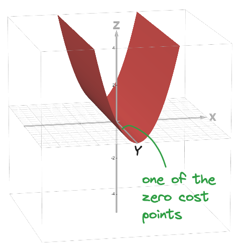
Source: https://www.desmos.com/3d (z=x²)
This surface contains all possible solutions to the problem. Although you can move in three orthogonal directions, you realize that only two specific dimensions (x and z) are crucial for solving the problem. Moving along the (y) dimension does not change the outcome or the cost of the solution. Once you reach the zero-cost point, any movement along the (y) dimension keeps the cost at zero, defining the solution set (s = 1) as illustrated in the above image.
The two dimensions that truly matter are referred to as the ID of the model for the given task, with ID = 2 in this case. This means that despite the apparent complexity of the 3D space, only two dimensions are essential in determining the solutions. When n = 3 and ID = 2, the problem and its solutions are effectively constrained to a two-dimensional subspace within the larger 3D space.
Let’s take another example: The function shows a non-convex landscape with 2 minima and maxima, illustrating the complexity of the optimization process in high-dimensional spaces.
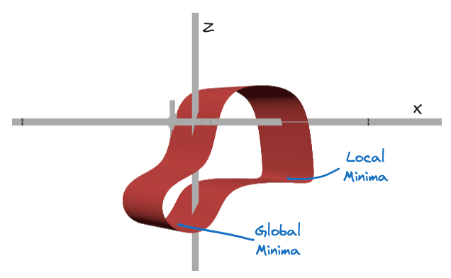
z=x²+z²+sin(3x)*cos(3z)+sin(x) in https://www.desmos.com/3d. The image is zoomed and inverted for a better view.
Despite the complexity, the ID remains 2, emphasizing that only x and z are required for achieving satisfactory solutions. Moving along the (y) dimension does not change the outcome or the cost of the solution. This shows that even in a non-convex space, understanding the ID helps simplify the optimization problem.
This concept becomes particularly relevant when (n) reaches millions, while the ID remains only in the hundreds. This relationship is expressed as (n = s + ID) where s represents the dimension (or cardinality) of the solution set. As (n) increases significantly, the idea of local minima becomes more complex, and the simple notion of a valley does not accurately represent the nature of high-dimensional spaces.
The surface of function in most dimensions is infinitely flat (Goodfellow et al.,)⁶ Not really hills and valleys.
In their seminal work, Li et al.,¹ demonstrate that a classifier with fully connected (FC) modules structured as 784–200–200–10 results in a total of n = 199,210 parameters. Through a series of experiments that systematically increase the subspace dimension d, they found that the subspace dimension at which performance exceeds the 90% threshold is approximately 750 on the MNIST dataset. This dimension is referred to as the network’s ID at the 90% performance mark, denoted as ‘d₉₀’.
How do you identify the ID of a network?
The most intuitive next question is: How do you choose these specific 750 parameters out of the 199,210 parameters? The answer is — you don’t. Instead of optimizing in the full n-dimensional space, the parameters are projected into a lower d-dimensional subspace. This approach freezes the majority of the n parameters and fine-tunes only d parameters.
Questions like How do you project the base model parameters (n) into the lower-dimensional space (d)?, How does this projection integrate into the network’s computation graph to allow gradients to flow? and Why does projection work? are explored in greater detail in Part 2.
If ID is so low why do we have such large networks in the first place?
Often the most accurate directly trained models for a problem have far more parameters than needed (Zhang et al.,)². This may be because they are just easier to train, and our observation suggests a reason why: with larger models, solutions have greater redundancy and in a sense “cover” more of the space (Li et al.)¹.
In the above 3D example, the zero-cost point can move freely along the y-dimension while still maintaining zero cost. This indicates that any point along the y-dimension is equally valid, as all these points represent zero cost. Consequently, there are multiple ways to achieve zero cost, and these solutions are effectively equivalent in terms of their performance.
In the case of above classifier example, there are 198,460 different directions in which one can move from a configuration which contributes to zero cost and remain at zero cost. These 198,460 parameters are added to the solution space. So, there’s a lot of flexibility in how you can arrive at a minimal cost solution. So the dummy parameters which increase the solution space actually help the training to converge faster.

Analogy to show multiple ways to reach the valley representing the zero cost. {Image Source: Gemini}
How does ID influence fine-tuning?
So far, we’ve understood that ID identifies the smallest number of parameters required for satisfactory solutions. Aghajanyan et al.³ looked at fine-tuning pre-trained models through the lens of ID and discovered that ID of pre-trained models is remarkably low.
For instance, with RoBERTa⁴ Large (354M parameters), fine-tuning only 207 parameters — less than 0.00006% of the total — achieved 90% of the model’s full performance on the MRCP⁵ dataset. Specifically:
Full fine-tuning (all 354M parameters) yielded an accuracy of 85%.
Fine-tuning just 207 parameters achieved 76.5% accuracy, which is 90% of the full parameterization’s performance.
This highlights that the ID at 90% performance (d₉₀) for this task is 207. Similar to the earlier discussion, this process does not involve selecting specific parameters; instead, the high-dimensional parameter space is projected into a lower-dimensional subspace. The authors used the Structure-Aware Intrinsic Dimension (SSID) method to determine d₉₀. During this process, the pre-trained model’s parameters remain frozen, and only the projected parameters are fine-tuned.
While subspace training itself performs fine-tuning, the novelty lies in developing algorithms that achieve fine-tuning efficiently — both in terms of performance and computation. This is where techniques like LoRA and similar algorithms stand out as differentiators.
Two takeaways from this work are:
Larger models are easier to fine-tune due to their low IDs.
Longer pre-training makes models easier to fine-tune, as they become better aligned with task-specific objectives.
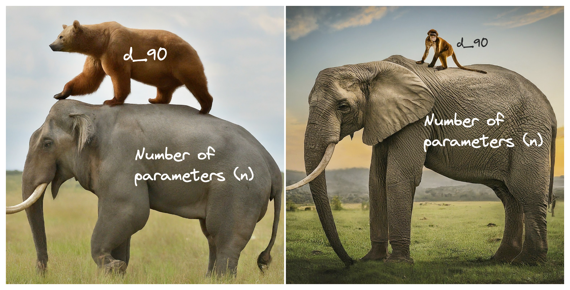
As the model size (n = number of parameters) increases, d_90 required for the fine-tuning task decreases. {Image Source: Gemini}
Why Does This Matter? Where Does It Lead?
Now that we understand fine-tuning large models with fewer parameters, it’s easier to appreciate adapter-based Parameter-Efficient Fine-Tuning (PEFT) methods. One such method, LoRA, introduces additional parameters called adapters, which are the only components trained during the fine-tuning process. The key idea is to fine-tune and save only these adapters for each downstream task, significantly reducing resource requirements.
For more details on LoRA, please refer to my previous blogs Idea behind PEFT and LoRA and Analyzing LoRA through its implementation on an MLP.
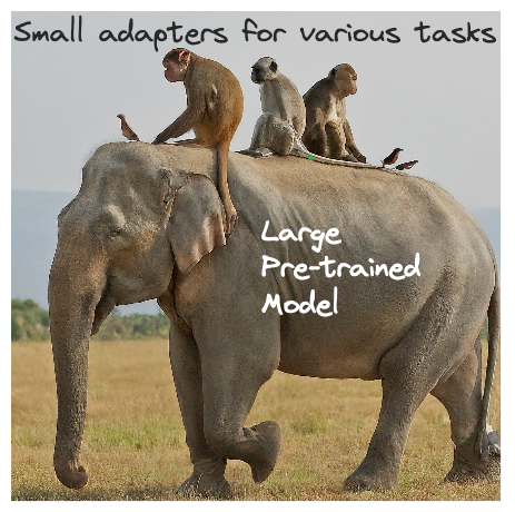
Multiple small adapters can be fine-tuned and stored over a large pre-trained model. {Image Source: Gemini}
Important Note: Typically, an n-dimensional equation requires an n+1-dimensional space for plotting, with the n+1ᵗʰ dimension representing the function’s value. Since plotting a function with 3 parameters would require a 4-dimensional space, which is difficult to visualize, I discounted the mathematical accuracy in order to better demonstrate the idea of ID.
In Part 2, we will demystify the process of measuring ID using random subspace training, as outlined in Section 2 of the referenced paper by Li et al.,¹. We will focus on the intricacies of the projection mechanism, systematically addressing key questions and replicating the results presented in the original work.
All images are by the author unless otherwise stated.
[1] Chunyuan Li and Heerad Farkhoor and Rosanne Liu and Jason Yosinski. Measuring the ID of Objective Landscapes, 2018.
[2] Chiyuan Zhang and Samy Bengio and Moritz Hardt and Benjamin Recht and Oriol Vinyals}. Understanding deep learning requires rethinking generalization}, 2017.
[4] Yinhan Liu, Myle Ott, Naman Goyal, Jingfei Du, Mandar Joshi, Danqi Chen, Omer Levy, Mike Lewis, Luke Zettlemoyer, Veselin Stoyanov. RoBERTa: A Robustly Optimized BERT Pretraining Approach, 2019

